How The Descent Was Made

Step one

The corpus: the essay's own words

The training data is a single passage of 2,402 characters — the essay distilled to its spine, from the first silence to hold it anyway. There is no other data. The model sees this text and nothing else, so whatever it learns, it learns from the argument it is standing inside.

The text is fed to the model one character at a time — not words, characters — and there are exactly 36 distinct ones across the whole passage (the letters it uses, a space, and a handful of marks). The model's only task is the humblest one imaginable: given the characters so far, guess the next.

Step two

The model: a very small transformer

The mind itself is a miniature GPT — the same architecture behind the large language models, shrunk until it fits in a coffee break. Three layers, four attention heads, a 64-dimensional inner representation, a context window of 64 characters. That is 158,820 trainable numbers in all: the entire being of this little reader.

# a tiny char-level GPT: 3 layers, 4 heads, 64 dims
class TinyGPT(nn.Module):
    def __init__(self):
        self.tok    = nn.Embedding(36, 64)      # 36 characters -> 64-d vectors
        self.pos    = nn.Embedding(64, 64)      # where in the window each one sits
        self.blocks = [Block() for _ in range(3)]   # 3 transformer layers
        self.head   = nn.Linear(64, 36)         # -> a probability for each next char

Every one of those 158,820 numbers begins as noise. Stacked into a single long list, they are a point in a space of 158,820 dimensions — and training is nothing more than moving that point, step by step, to a place where the essay looks less surprising.

Step three

Training, and photographing the fall

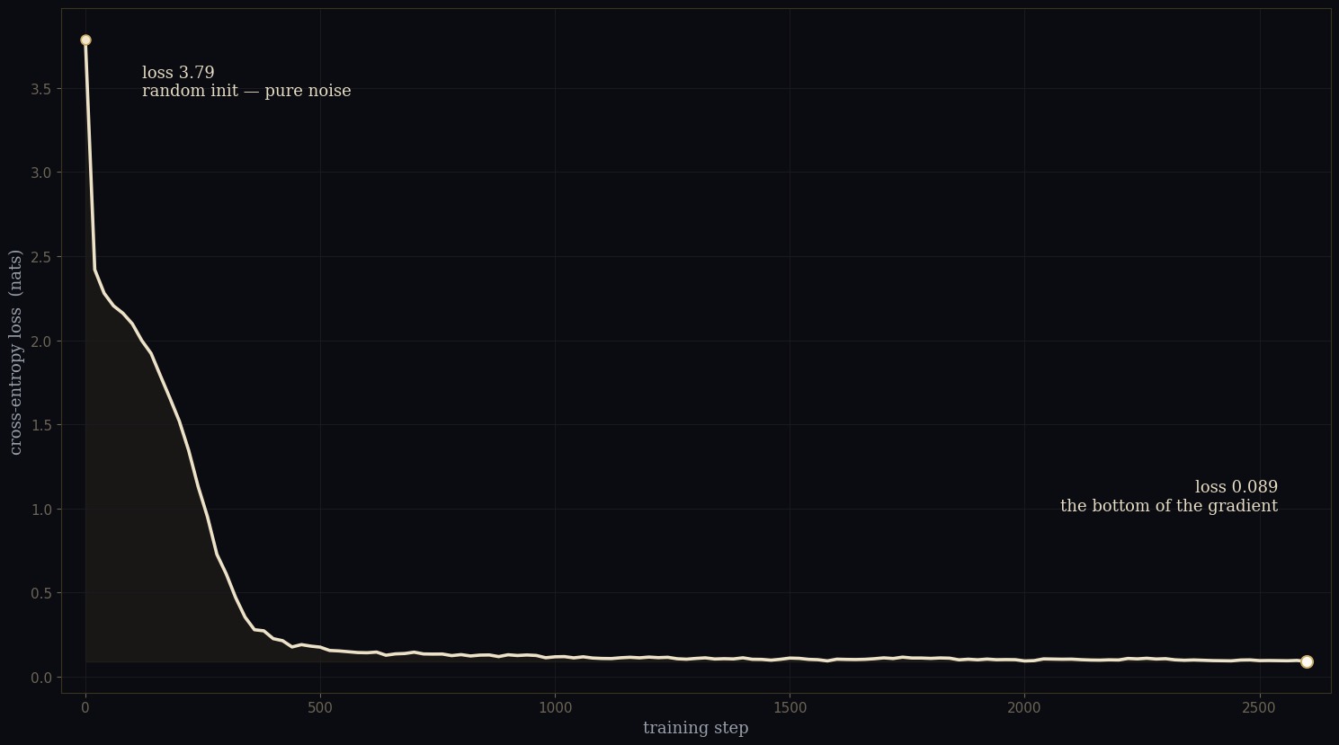
The model is trained by ordinary gradient descent: show it a batch of the text, measure how wrong its next-character guesses are (the loss), compute which way to nudge each of the 158,820 numbers to be a little less wrong, and take the step. Two thousand six hundred times. It takes about half a minute on a single graphics card.

The crucial move for the picture comes here: every twenty steps, the model's entire parameter vector is saved — a full photograph of where the point currently sits in its 158,820-dimensional space. That gives 131 snapshots, a frame-by-frame record of the exact route the optimizer walked.

opt = torch.optim.AdamW(model.parameters(), lr=3e-3)
for step in range(2601):
    if step % 20 == 0:                 # every 20 steps...
        snaps.append(get_flat())       # ...save all 158,820 numbers
        curve.append(eval_loss())      # ...and the loss right now
    x, y = get_batch()                 # a batch of the essay
    _, loss = model(x, y)
    loss.backward(); opt.step()        # the descent, one step

Measured on a fixed slice of the text so the numbers are comparable, the loss falls from 3.79 — the pure confusion of random initialization, barely better than guessing among 36 characters blind — to 0.089, near-perfect recall of the passage. That fall is the whole story, and it looks like this:

Step four

The problem: you cannot draw 158,820 dimensions

Here is the honest difficulty. The loss is a landscape — a height (how wrong the model is) over a terrain of every possible setting of its numbers. But that terrain has 158,820 dimensions, and a page has two. There is no way to simply look at it. Almost every attempt to picture a loss landscape quietly cheats at this step, drawing a suggestive bowl and hoping you do not ask what its axes mean.

The path out is a published technique (Li et al., 2018, building on Goodfellow): instead of choosing two axes arbitrarily, let the optimizer's own trajectory choose them. The route it walked lives, it turns out, almost entirely in a flat two-dimensional plane inside that vast space. Find that plane, and you are drawing the loss on the exact window the descent actually happened in — not a decorative slice, but the right one.

Step five

Finding the plane the optimizer fell through

The plane is built from the 131 snapshots. Its first axis is chosen deliberately: the straight line from where training started to where it ended — the true fall line, the net direction of the whole descent. The second axis is whatever remaining direction the path wandered in most, recovered by a standard decomposition (PCA) of the trajectory once the fall line is removed.

W = np.stack(snaps)                     # (131 snapshots, 158820 numbers)
u = theta_final - theta_init            # axis 1: the fall line
u /= np.linalg.norm(u)                  #   where it actually ended up
resid = Dm - np.outer(Dm @ u, u)        # strip the fall-line part away
_, _, Vt = np.linalg.svd(resid)         # axis 2: the main lateral wander
PC = np.stack([u, Vt[0]])               # the plane the descent lived in

Choosing the fall line as the first axis is what makes the picture a plunging valley rather than a flat, ambiguous saddle: it points the camera straight down the direction the loss actually dropped. And it is faithful, not cherry-picked — projected onto this one plane, the 131 real snapshots retain 90.3% of their total movement. The optimizer really did travel, almost entirely, in this two-dimensional window.

Step six

Measuring the real surface, one point at a time

Now the surface. For each point on a 46×46 grid laid across that plane, the model's parameters are physically set to that point — θ = θ_final + a·axis₁ + b·axis₂ — and the actual loss is measured by running the essay through the model there. Not interpolated, not guessed: 2,116 real forward passes of a real network. That is the height of the land at every point.

# evaluate the REAL loss on a 46 x 46 grid in the plane
for b in B:
    for a in A:
        set_flat(theta_final + a*PC[0] + b*PC[1])   # move the model here
        Z[i, j] = eval_loss()                       # measure its real loss

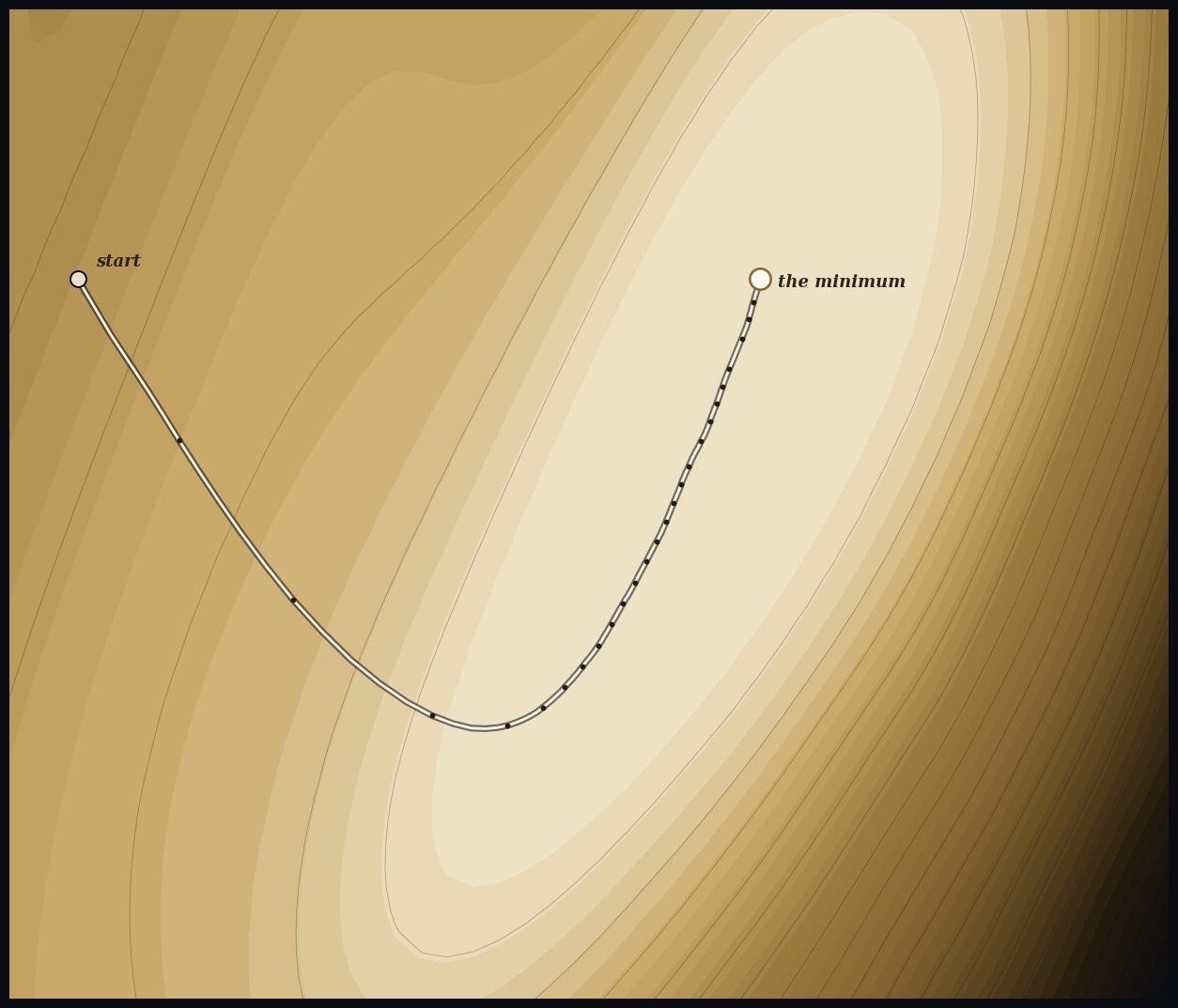
The grid is stretched a little past the endpoint on the downhill side, so the far walls of the valley rise into view; measured loss ranges from 0.086 at the floor to almost 15 up the sides. Finally the 131 trajectory snapshots are projected onto the same plane and laid on the surface at their true heights — the glowing thread you see descending. Seen from directly above, the plane and the path look like this:

Step seven

Rendering: gold on deep space

Only the last step is aesthetic, and it changes no number. The measured height-field is lit as a relief — low loss glows, the high walls fall into shadow — painted in the essay's own palette of gold on deep space, with a topographic contour map cast on the floor beneath. The real trajectory is drawn as a bright thread that grows in across the turn, with small chevrons marking the direction of the fall, and the whole surface is spun a slow 360° so the valley reads as a valley from every side.

What turns, then, is a measurement. The bowl is where the network's error actually is; the thread is where its optimizer actually went; the bottom of the valley is the passage above, very nearly memorized.

Reproduce it

Run the descent yourself

The whole thing is two small Python scripts and about a minute of compute. The first trains the model, captures the trajectory, and measures the surface; the second lights and spins it.

# train the mind on the essay, capture the real loss landscape
python descent.py            # -> captures/descent.npz

# light it, draw the real path, spin it 360°
python render_turntable.py   # -> descent_turntable.mp4

Everything is deterministic (the random seed is fixed at 1337), so the same commands yield the same descent, the same plane, the same figure, every time. That reproducibility is the point: the picture is not an artist's impression of the idea in Movement IV. It is the idea, executed and measured, and the measurement is the same whoever runs it.